Impulses of electric current of a certain preset. Electrical impulses and their parameters
Under electrical impulse understand the deviation of voltage or current from a certain constant level (in particular, from zero), observed for a time less than or comparable to the duration of transients in the circuit.
As already mentioned, the transient process is understood as any abrupt change in the steady state in an electrical circuit due to the action of external signals or switching within the circuit itself. Thus, the transient process is the process of the transition of an electrical circuit from one stationary state to another. No matter how short this transitional process is, it is always finite in time. For circuits in which the lifetime of the transient process is incomparably shorter than the duration of the external signal (voltage or current), the operating mode is considered steady, and the external signal itself for such a circuit is not pulsed. An example of this would be the actuation of an electromagnetic relay.
When the duration of voltage or current signals acting in the electric circuit becomes commensurate with the duration of the establishment processes, the transient process has such strong influence on the shape and parameters of these signals, so that they cannot be ignored. In this case, most of the time the signal is applied to the electrical circuit coincides with the time of the transient process (Figure 1.4). The operating mode of the circuit during the action of such a signal will be non-stationary, and its impact on the electrical circuit will be impulsive.
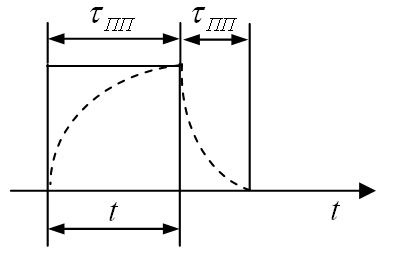
Figure 1.4. The relationship between signal duration and duration
transition process:
a) the duration of the transient process is much shorter than the duration
signal ( τ pp<< t );
b) the duration of the transient process is commensurate with the duration
signal ( τ пп ≈ t ).
Hence it follows that the concept of a pulse is associated with the parameters of a particular circuit and that not for every circuit the signal can be considered as pulsed.
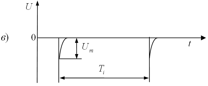
Thus, an electrical impulse for a given circuit is the voltage or current acting for a period of time commensurate with the duration of the transient in this circuit. In this case, it is assumed that there must be a sufficient time interval between two consecutive pulses in the circuit, exceeding the duration of the settling process. Otherwise, instead of pulses, signals of complex shape will appear (Fig. 1.5).
Figure 1.5. Complex electrical signals
The presence of time intervals imparts a characteristic discontinuous structure to the impulse signal. Some conventionality of such definitions lies in the fact that the process of establishment theoretically lasts forever.
There may be such intermediate cases when the transient processes in the circuits do not have time to practically end from pulse to pulse, although the acting signals continue to be called pulsed. In such cases, additional distortions of the pulse shape occur, caused by the superposition of the transient process at the beginning of the next pulse.
There are two types of impulses: video pulses and radio pulses ... Video pulses are received when switching (switching) a DC circuit. Such pulses do not contain high-frequency oscillations and have a constant component (average value) other than zero.
Video pulses are usually distinguished by their shape. In fig. 1.6. the most common video pulses are shown.


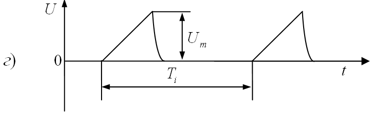


Rice. 1.6. Video pulse shapes:
a) rectangular; b) trapezoidal; v) spiky;
G) sawtooth; e) triangular; e) opposite polarity.
Consider the main parameters of a single pulse (Figure 1.7).

Rice. 1.7. Single pulse parameters
The shape of the pulses and the properties of its individual sections are quantitatively assessed by the following parameters:
· U m - the amplitude (highest value) of the pulse. Pulse amplitude U m (I m) expressed in volts (amperes).
· τ and - pulse duration. Usually, measurements of the duration of pulses or individual sections are made at a certain level from their base. If this is not specified, then the pulse duration is determined at the zero level. However, most often the pulse duration is determined at the level 0.1U m or 0.5U m counting from the base. In the latter case, the pulse duration is called active duration and denoted τ and ... If necessary and depending on the shape of the impulses, the accepted level values for measurement are specially negotiated.
· τ f - rise time, determined by the rise time of the pulse from the level 0.1U m to level 0.9U m .
· τ with - the duration of the cutoff (trailing edge), determined by the decay time of the pulse from the level 0.9U m to level 0.1U m ... When the duration of the rising or falling edge is measured at the level 0.5U m , it is called the active duration and is indicated by the addition of the index "a" similar to active pulse width. Usually τ f and τ with is a few percent of the pulse duration. The less τ f and τ with compared with τ and , the more the shape of the pulse approaches rectangular. Sometimes instead of τ f and τ with pulse fronts are characterized by the rate of rise (fall). This value is called steepness (S) of the front (cut) and expressed in volts per second (V/with) or kilovolts per second (kV/with) ... For rectangular pulse
 ………………………………(1.14).
· The section of the pulse between the fronts is called a flat top. Figure 1.7 shows the decline of a flat top (ΔU) .
· Pulse power. Energy W the pulse, related to its duration, determines the power in the pulse:
 ………………………………(1.15).
It is expressed in watts (W) , kilowatts (kw) or fractional units
tsach watt.
Pulse devices use pulses with durations from fractions of a second to nanoseconds. (10 - 9 s) .
The characteristic sections of the impulse (Figure 1.8), which determine its shape,
are:
Front (1 - 2);
Top (2 - 3);
· Cut (3 - 4), sometimes called the trailing edge;
Tail (4 - 5).
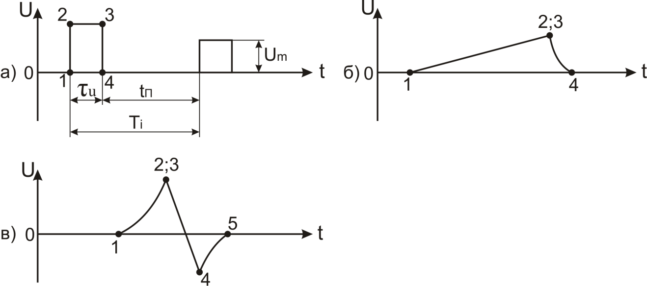
Figure 1.8. Typical pulse sections
Separate areas of impulses of various shapes may be absent. It should be borne in mind that real impulses do not have a form that strictly corresponds to the name. Distinguish between impulses of positive and negative polarity, as well as bilateral (oppositely polar) impulses
(fig. 1.6, e).
Radio pulses are pulses of high-frequency voltage or current fluctuations, usually sinusoidal. Radio pulses do not have a constant component. Radio pulses are obtained by modulating high-frequency sinusoidal oscillations in amplitude. In this case, amplitude modulation is performed according to the law of the control video pulse. The shapes of the corresponding radio pulses obtained using amplitude modulation are shown in Fig. 1.9:

Figure 1.9. Forms of radio pulses
Electrical impulses following each other at regular intervals are called periodic sequence (Figure 1.10).
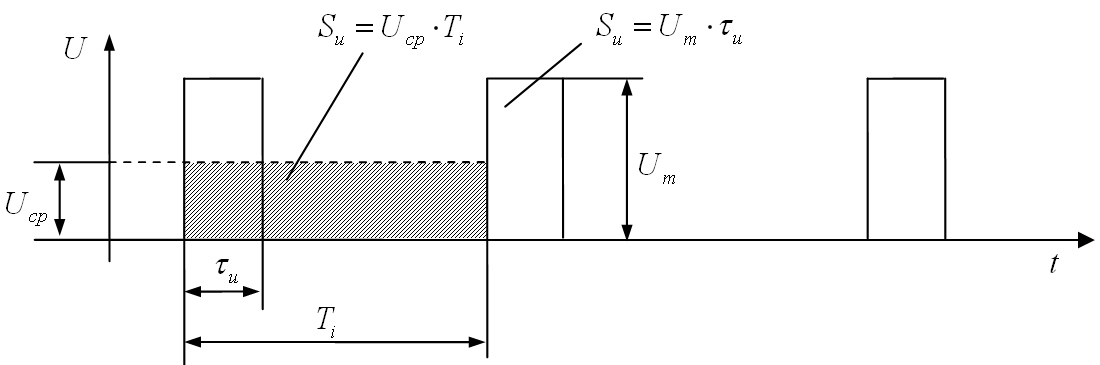
Figure 1.10. Periodic pulse train
The periodic sequence of pulses is characterized by the following parameters:
Repetition period T i - the time interval between the beginning of two adjacent unipolar impulses. It is expressed in seconds (with) or sub-multiples of a second (ms; μs; ns). The reciprocal of the repetition period is called the pulse repetition (repetition) frequency. It determines the number of pulses in one second and is expressed in hertz (Hz) , kilohertz (kHz) etc.
 ……………………………….. (1.16)
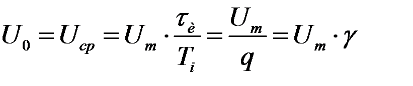
· The duty cycle of a pulse train is the ratio of the repetition period to the pulse width. Denoted by a letter q :
 ………………… (1.17)
The duty cycle is a dimensionless quantity that can vary over a very wide range, since the pulse duration can be hundreds or even thousands of times less than the pulse period, or, conversely, occupy most of the period.
The reciprocal of the duty cycle is called the duty cycle. This quantity is dimensionless, less than one. It is denoted by the letter γ :
 …………………………(1.18)
Pulse train with q = 2 called Meander ... Such
sequences  (Figure 1.6, e). If Т i >> τ and
, then such a sequence is called radar.
(Figure 1.6, e). If Т i >> τ and
, then such a sequence is called radar.
· Average value (constant component) of impulse fluctuations. When determining the average value of the impulse oscillation over the period U Wed (or I Wed) the voltage or current pulse is distributed evenly over the entire period so that the area U cf · T i was equal to the pulse area S u = U m τ and (fig. 1.10).
For pulses of any shape, the average value is determined from the expression
 ……………………(1.19),
where U (t) is an analytical expression for the pulse shape.
For a periodic sequence of pulses rectangular, in which U (t) = U m , repetition period T i and pulse duration τ and , this expression after substitution and transformation takes the form:
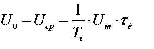 …………………….(1.20).
Fig. 1.10 it is seen that S u = U m τ and = U cf · T i , whence follows:
 ……………(1.21),
where U 0 - is called a constant component.
Thus, the average value (constant component) of the voltage (current) of the sequence of rectangular pulses in q times less than the pulse amplitude.
· Average power of the pulse train. Pulse energy W related to the period T i , determines the average pulse power
 …………………………….. (1.22).
Comparing expressions P and and P Wed , we get
P u τ u = P cf T i ,
whence follows
 …………………(1.23)
and  ……………………. (1.24),
those. average power and pulse power differ in q once.
From this it follows that the pulse power provided by the generator can be q times the average power of the generator.
Tasks and exercises
1. The pulse amplitude is 11 kV, the pulse duration is 1 µs. Determine the slope of the leading edge of the pulse if the rise time is assumed to be 20% of the pulse width.
2. The amplitude of rectangular pulses with a repetition rate of 1250 Hz and a duty cycle of 2300 is 11 kV. Determine the slope of the leading edge and the cutoff, assuming the rise and fall times are equal to 20% of the pulse duration.
3. Determine the time constant of a circuit consisting of a 5000 pF capacitor and an active resistance of 0.5 MΩ.
4. Determine the time constant of the circuit consisting of an inductance of 20 mH and an active resistance of 5 kOhm.
5. Determine the average power of the radar transmitting device, which has the following parameters: pulse power 800 kW; the duration of the probe pulse is 3.2 μs; the repetition rate of the probing pulses is 375 Hz.
6. A 400 pF capacitor is charged from a 200 V constant voltage source through a 0.5 MΩ resistance. Determine the voltage across the capacitor 600 μs after the start of charging.
7. To the circuit, consisting of a capacitor with a capacity of 10 pF and a resistance of 2 MΩ, a direct current source with a voltage of 50 V is connected. Determine the current at the moment of switching on and 40 μs after switching on.
8. A capacitor charged to a voltage of 300 V is discharged through a 300 MΩ resistance. Determine the value of the discharge current over time t = 3τ after the start of the discharge.
9. How long will it take to charge a 100 pF capacitor to a voltage of 340 V, if the voltage of the source is 540 V and the resistance of the charging circuit is 100 kΩ?
10. The circuit, consisting of an inductance of 10 mH and a resistance of 5 kOhm, is connected to a constant voltage source of 250 V. Determine the current flowing in the circuit 4 μs after switching on.
Chapter 2. Pulse shaping
Linear and non-linear circuits
In pulsed technology, circuits and devices are widely used that form voltages of one form from the voltage of another. Such problems are solved using linear and non-linear elements.
An element whose parameters (resistance, inductance, capacity) do not depend on the magnitude and direction of currents and applied voltages is called linear. Circuits containing linear elements are called
linear.
Linear circuit properties:
· The current-voltage characteristic (VAC) of a linear circuit is a straight line, i.e. the values of currents and voltages will be related to each other by linear equations with constant coefficients. An example of a CVC of this type is Ohm's law:  .
.
· For the calculation (analysis) and synthesis of linear circuits, we apply the principle of superposition (overlay). The meaning of the principle of superpositions is as follows: if a sinusoidal voltage is applied to the input of a linear circuit, then the voltage on any of its elements will have the same shape. If the input voltage is a complex signal (that is, it is the sum of harmonics), then all the harmonic components of this signal are preserved on any element of the linear circuit: in other words, the shape of the voltage applied to the input is preserved. In this case, only the ratio of harmonic amplitudes will change at the output of the linear circuit.
· The linear circuit does not convert the spectrum of the electrical signal. It can change the components of the spectrum only in amplitude and phase. This is the reason for the occurrence linear distortion .
· Any real linear circuit distorts the waveform due to transients and finite bandwidth.
Strictly speaking, all elements of electrical circuits are non-linear. However, in a certain range of variation of variable values, the nonlinearity of the elements appears so little that it can be practically neglected. An example is a radio frequency amplifier (RF amplifier) of a radio receiver, to the input of which a signal from an antenna is very small in amplitude.
The nonlinearity of the input characteristics of the transistor in the first stage of the RF amplifier is so small within a few microvolts that it is simply not taken into account.
Usually, the area of nonlinear behavior of an element is limited, and the transition to nonlinearity can occur either gradually or in a jump.
If a complex signal is applied to the input of a linear circuit, which is the sum of harmonics of different frequencies, and the linear circuit contains a frequency-dependent element ( L or C ), then the shape of the voltages on its elements will not repeat the shape of the input voltage. This is because the harmonics of the input voltage are passed differently by such a circuit. As a result of the passage of the input signal through the capacitances and inductances of the circuit, the relationship between the harmonic components on the circuit elements changes in amplitude and phase with respect to the input signal. As a result, the relationships between the amplitudes and phases of the harmonics at the input to the circuit and at its output are not the same. This property is the basis for the formation of pulses using linear circuits.
An element, the parameters of which depend on the magnitude and polarity of the applied voltages or flowing currents, is called nonlinear , and a chain containing such elements is called nonlinear .
Nonlinear elements include electrovacuum devices (EVD), semiconductor devices (PPP) operating in the nonlinear section of the I – V characteristic, diodes (vacuum and semiconductor), as well as transformers with ferromagnets.
Nonlinear circuit properties:
· The current flowing through the nonlinear element is not proportional to the voltage applied to it, i.e. the relationship between voltage and current (VAC) is non-linear. An example of such a CVC is the input and output characteristics of the EEC and the RFP.
Processes in nonlinear circuits are described by nonlinear equations of various kinds, the coefficients of which depend on the voltage (current) function itself or on its derivatives, and the I - V characteristic of a nonlinear circuit has the form of a curve or a broken line. An example is the characteristics of diodes, triodes, thyristors, zener diodes, etc.
· For nonlinear circuits, the principle of superposition is not applicable. When an external signal acts on nonlinear circuits, currents always appear in them, containing in their composition new frequency components that were not in the input signal. This is the reason for the occurrence
nonlinear distortion , as a result of which the signal at the output is nonlinear
the circuit is always different in shape from the input signal.
Differentiating circuits
To gain momentum desired shape from a given voltage form using a passive electrical circuit, it is necessary to know the forming properties of this circuit. Forming properties characterize the ability of a linear circuit to change the shape of the transmitted (processed) signal in a certain way and are completely determined by the type of its frequency and time. NS x characteristics.
In pulse technology, linear two- and four-port networks are widely used to generate signals.
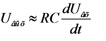
Differentiating called a circuit, at the output of which the voltage is proportional to the first derivative of the input voltage. Mathematically, this is expressed by the following formula:
 ………………………. (2.1),
where U in - voltage at the input of the differentiating circuit;
U out- voltage at the output of the differentiating circuit;
k - coefficient of proportionality.
Differentiating circuits (DC) are used to differentiate video pulses. At the same time, the differentiating circuits allow the following transformations:
· Shortening of rectangular video pulses and the formation of sharp-pointed pulses from them, which serve to trigger and synchronize various pulse devices;
· Obtaining time derivatives of complex functions. It is used in measuring technology, auto-control systems and auto-tracking;
· Formation of rectangular impulses from sawtooth.
The simplest differentiating circuits are capacitive ( RC ) and inductive ( RL ) chains (Figure 2.1):


Figure 2.1. Types of differentiating circuits:
a) capacitive DC; b) inductive DC
Let us show that RC - the chain becomes differentiating under certain conditions.
It is known that the current flowing through the capacitor is determined by the expression:
 ........................................... (2.2).
At the same time, from Figure 2.1, a it's obvious that
 ,
,
since R and C represent a voltage divider. Since the voltage
 , then .
Output voltage
 ………………….... (2.3).
Substituting expression (2.2) into (2.3), we obtain:
 ……………… (2.4).
If we choose a sufficiently small value R so that the condition is met,
then we get an approximate equality
 ……………………….. (2.5).
This equality is identical to (2.1).
Select R sufficiently small - this means to ensure the fulfillment of the inequality
where ω in = 2πf in - the upper cutoff frequency of the output signal harmonic, which still has essential for the output pulse shape.
The proportionality coefficient in expression (2.1) k = RC = τ bears the name time constant differentiating circuit. The more abruptly the applied voltage changes, the smaller the value τ must have a differentiating circuit so that the voltage at the output is close in shape to the derivative of U in ... Parameter τ = RC has the dimension of time. This can be confirmed by the fact that, in accordance with the International System of Units (SI), the unit of measurement for electrical resistance
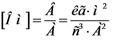 ,
,
and the unit of measurement for electrical capacity
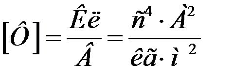 .
.
Hence,

The principle of operation of the differentiating circuit.
A schematic diagram of a capacitive differentiating circuit is shown in Figure 2.2, and the voltage diagrams are shown in Figure 2.3.
![]()
Figure 2.2. Schematic diagram of a capacitive differentiating circuit
Let an ideal rectangular impulse be applied to the input, for which
τ ф = τ с = 0, a internal resistance signal source R i = 0 .Let the momentum be determined by the following expression:

- The initial state of the circuit (t< t 1).
In its original state U in = 0; U with = 0; i with = 0; U out = 0.
- First voltage jump (t = t 1).
At the moment of time t = t 1, a voltage jump is applied to the DC input
U in = E... In this moment U c = 0 since for an infinitely small period of time, the capacity cannot be charged. But, in accordance with the law of commutation, the current through the capacitor can increase instantly. Therefore, at the moment t = t 1, the current flowing through the capacitor will be equal to

Therefore, the voltage at the output of the circuit at this moment will be equal to

- Capacitor charge (t 1< t < t 2).
After the jump, the capacitor begins to charge with a current that decreases exponentially:
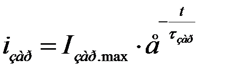

Figure 2.3. Diagrams of stresses on the elements of the differentiating circuit
The voltage across the capacitor will grow exponentially
 …………………… (2.6).
The voltage at the output of the DC will drop as the voltage rises
charge on the capacitor, because R and C represent a voltage divider:
 …………. (2.7).
It must be remembered that at any time for the voltage divider the equality
whence it follows that
which confirms the validity of expression (2.7).
Theoretically, the charge of the capacitor will continue for an infinite time, but in practice this transient process ends after
(3…5)τ charge
= (3…5)RC
. 
- End of capacitor charging (t = t 2).
After the end of the transient process, the capacitor charge current becomes zero. Therefore, the voltage at the output of the differentiating circuit

reaches almost zero value, i.e. at time t = t 2


- Steady-state mode (t 2< t < t 3).
Wherein 


- Second voltage jump (t = t 3).
At a moment in time t = t 3
the voltage at the input of the differentiating circuit drops abruptly to zero. Capacitor C
becomes a source of tension, because it is charged to the magnitude  .
.
Since, in accordance with the law of commutation, the voltage across the capacitor cannot change abruptly, and the current flowing through the capacitor can change abruptly, then at the moment t = t 3 the output voltage drops abruptly to – E ... In this case, the discharge current in this moment time becomes maximum:
 ,
,
and the voltage at the output of the differentiating circuit
 .
.
The output voltage has a minus sign, because the current has changed its direction.
- Capacitor discharge (t 3< t < t 4).
After the second jump, the voltage across the capacitor begins to decrease exponentially:
 ;
;  ;
; 
- The end of the capacitor discharge and the restoration of the initial state of the circuit (t≥ t 4).
After the end of the transient process of the discharge of the capacitor

Thus, the circuit returned to its original state. The end of the capacitor discharge occurs practically at t = (3… 5) τ = (3… 5) RC.
Since we took the internal resistance of the signal source R i = 0, then we can assume that the time constants of the charge and discharge circuits of the capacitor τ charge = τ times = τ =RC .
In such an ideal circuit, the amplitude of the output voltage U out. m ah does not depend on the value of the circuit parameters R and C , and the duration of the pulses at the output is determined by the value of the circuit time constant τ = RC ... The smaller the value R and C , the faster the transient processes of charge and discharge of the capacitance end, the shorter the pulse at the output of the circuit.
Theoretically, the duration of the pulse at the output of the differentiating circuit, determined from the base, turns out to be infinitely long, since the voltage at the output drops exponentially. Therefore, the pulse duration is determined at a certain level from the base
U 0 = αU out (Figure 2.4):

Figure 2.4. Determination of the pulse duration at the level U 0 after
differentiation
Let us determine the duration of the differentiated pulse at the level
U 0 = αU out :
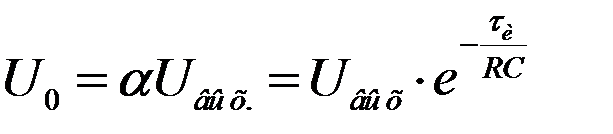 ………………. (2.8),
where  and
and  ……………………… (2.9).
Differentiation is always accompanied by a shortening of the pulse width. This means that the capacity C must have time to fully charge during the time of the current input differentiable pulse. Consequently, the condition for practical differentiation in order to shorten the pulse duration is the ratio:
τ and in> 5τ = 5RC.
The less τ circuit, the faster the capacitor is charged and discharged and the shorter the duration of the output pulses, the more spiky they become and, therefore, the more accurate the differentiation. However, reduce τ expedient up to a certain limit.
The change in the shape of the pulse at the output of the differentiating circuit can be explained in terms of spectral analysis.
Each harmonic of the input pulse is divided between R and C ... For harmonics low frequencies determining the top of the input pulse, the capacitor presents a large resistance, since
 >> R
.
>> R
.
Therefore, the flat top of the input pulse is hardly transmitted to the output.
For the high-frequency components of the input pulse, which form its leading edge and cutoff,
 << R
.
<< R
.
Therefore, the front and edge of the input pulse are transmitted to the output practically without attenuation. These considerations make it possible to define the differentiating circuit as high pass filter .
Electric impulse, short-term change in electrical voltage or current. Short is understood as a period of time comparable to the duration transient processes in electrical circuits ... I. e. divided into high-voltage pulses, high-strength current pulses, video pulses and radio pulses. I. e. high voltages are usually obtained during the discharge of a capacitor to a resistive load and have an aperiodic shape. Lightning strikes usually have the same shape. Solitary I. e. of a similar shape with an amplitude of several sq. up to several Mv with a wave front 0.5-2 microseconds and duration 10-10 -2 microseconds used for testing electrical devices and equipment in high voltage technology. Current jumps of high strength can be similar in shape to I. e. high voltage (see. Impulse technique high voltages).
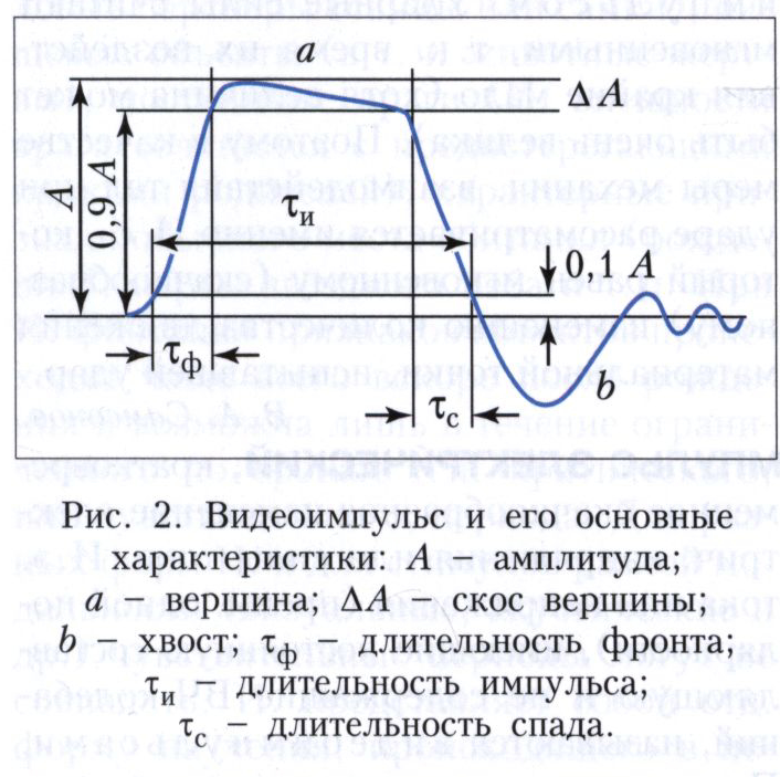
Video pulses are called I. e. current or voltage (mainly of the same polarity), having a constant component other than zero. Distinguish between rectangular, sawtooth, trapezoidal, exponential, bell-shaped and other video pulses ( rice. 1 , a-d). The characteristic elements that determine the shape and quantitative parameters of the video pulse ( rice. 2 ) are the amplitude A, the front t f, the duration t and, the decay t c and the slope of the top (D A), usually expressed in% of A. ... Duration of video pulses - from fractions sec to tenths nsec (10 -9 sec). Video pulses are used in television, computer technology, radar, experimental physics, automation, etc.
Intermittent HF or UHF oscillations of electric current or voltage ( rice. 1 , e), the amplitude and duration of which depend on the parameters of the modulating oscillations. The duration and amplitude of the radio pulses correspond to the parameters of the modulating video pulses; additional parameter - carrier frequency. Radio pulses are used mainly in radio and communication technology. The duration of radio pulses is in the range from fractions sec before nsec.
Lit .: Itskhoki Ya. S., Impulse devices, M., 1959; Fundamentals of impulse technology, M., 1966; Brammer Yu.A., Pashchuk I.N., Impulse technique, 2nd ed., M., 1968.
Great Soviet Encyclopedia M .: "Soviet Encyclopedia", 1969-1978
Typical examples of rectangular pulses are primary telegraph and data signals, also called DC pulses. They have the form of sequences of bipolar or unipolar rectangular pulses (Fig. 6.1, a).
Let us find the spectrum of a periodic sequence of unipolar pulses with a period and amplitude UQ. Such a sequence can be represented as a Fourier series:

where is the circular repetition rate or the first harmonic (spectral component) of the signal

Rice. 6.1 Pulse train (a) and its spectrum (b)
The coefficients determine the so-called amplitude spectrum, and the phase spectrum. Wherein
![]()
where is the duty cycle of the pulse sequence. Constant component or average value of the signal over the period.The amplitude spectrum for the case is shown in Fig.
The spectrum of a periodic sequence of unipolar pulses at contains, in addition to the constant component, components with frequencies, etc. The difference between these spectral components (decreases with increasing T, while the components themselves also decrease in amplitude. At, the signal becomes non-periodic, and the spectrum becomes continuous. Instead of the concept In this case, the concept of spectral density is introduced.The spectral density is defined as the ratio of the "amplitude of the spectral component" to the infinitesimal frequency band and is calculated through the Fourier integral:

where is the spectral density of the amplitudes; - spectrum of phases.
Knowing it can be found using the inverse Fourier transform:

The spectral density of the amplitudes of a single rectangular pulse up to a factor is shown by the dashed line in Fig.
The spectrum of a periodic sequence of pulses and a single pulse contains components with a frequency from 0 to infinity, that is, it is infinite. If a rectangular pulse train is transmitted over a communication channel that always passes only a limited spectrum, then the waveform at the output of the channel changes. The waveform can be determined using the inverse Fourier transform (6.6).
In practice, the bandwidth of the signal is usually understood as the frequency range in which the main signal energy is concentrated. In this case, the concept of the effective width of the signal spectrum is introduced. In fig. - this is the frequency range from 0 to in which about 90% of the signal energy is concentrated. This means that the shorter the pulse duration (the higher the telegraphy speed), the wider the spectrum. In particular, an infinitely short pulse has an infinitely extended spectrum with a uniform density. Thus, higher speed transmission requires higher bandwidth channels.
For a given duration of a unit element, two factors influence the spectrum of the transmitted signal. One is the pulse shape, which must be carefully selected to obtain a good (compact) signal spectrum. Another factor is the nature of the transmitted digital sequence, i.e. the spectrum depends on the statistical characteristics of the transmitted sequence, and the spectrum can be changed by recoding it.
To evaluate the spectrum clipping distortion of DC pulses, consider the passage of a pulse through an ideal low-pass filter (LPF). As an input we will use the step function
presented graphically in Fig. 6.2. The choice of such an input action is due to the fact that, firstly, its use simplifies mathematical calculations, and secondly, a single rectangular pulse of finite duration can be represented as a sequence of two single voltage surges of the opposite sign, shifted in time by an amount equal to the pulse duration (Fig. . 6.3).
Rice. 6.2 Step function
Rice. 6.3. Single pulse representation

Rice. 6.4. Characteristics of an ideal low-pass filter
And, finally, knowing the characteristics of the settling process under the action of a single jump, using the convolution theorem, one can find the settling process for an arbitrary form of action.
Let at the input of an ideal low-pass filter with a cutoff frequency, the amplitude and phase-frequency characteristics of which have the form (Fig.6.4):

where is the group time of the filter, at the moment the signal (6.7) is supplied, which can be represented in the form

To obtain the signal at the output of the low-pass filter, we multiply all the components of the input signal by the modulus of the filter gain and subtract the phase shift at each of the frequencies from the sine argument:
Substituting in (6.9) the value of the transmission coefficient from (6.8), we obtain
ELECTRIC IMPULSE, short-term abrupt change in electrical voltage or current. An electric current or voltage pulse (mainly of the same polarity) that has a constant component and does not contain HF oscillations are called video pulses. By the nature of the change in time, video pulses are distinguished of rectangular, sawtooth, trapezoidal, bell-shaped, exponential and other shapes (Fig. 1, a-d). A real video pulse can have a rather complex shape (Fig. 2), which is characterized by amplitude A, duration τ И (measured at a predetermined level, for example, 0.1 A or 0.5 A), duration of rise time τ Ф and decay τ С (measured between the levels of 0.1 A and 0.9 A), the bevel of the top ΔA (expressed as a percentage of A). The most widely used are rectangular video pulses, on the basis of which synchronization, control and information signals are formed in computer technology, radar, television, digital transmission and information processing systems, etc. , as well as in the formation of complex radar signals with intra-pulse frequency modulation. The duration of video pulses ranges from fractions of a second to tenths of a nanosecond.
In addition to single and irregularly following flows of electrical pulses in practice, periodic sequences are used, which are additionally characterized by a period T or a repetition frequency f = T -1. An important parameter of the periodic sequence of electrical pulses is the duty cycle (the ratio of the pulse repetition period to their duration). According to the frequency distribution, electrical pulses are characterized by a spectrum, which is obtained as a result of the expansion of a time function expressing an electrical pulse in a Fourier series (for a periodic sequence of identical pulses) or a Fourier integral (for single pulses).
Electric pulses, which are time-limited (intermittent) HF or microwave oscillations, the envelope of which is in the form of a video pulse (Fig. 1, e), are called radio pulses. The duration and amplitude of the radio pulses correspond to the parameters of the modulating video pulses; an additional parameter is the carrier frequency. Radio pulses are used mainly in radio and communication devices; their duration ranges from fractions of a second to several nanoseconds.
Lit .: Erofeev Yu. N. Impulse devices. 3rd ed. M., 1989; Brammer Yu. A., Pashchuk I. N. Impulse technique. M., 2005.